It's a data thing

In this post I want to show you how python can be used for a physics data analysis instead of the more widely used ROOT. Even though ROOT has its advantages when it comes to processing large datasets on the computing grid, running it on your personal computer can often be tedious. Python gives you a verity of tool, helpful especially in the late analysis stage, e.g. for creating plots or tables.

During CHEP 2018 Jim Pivarski gave a talk where he presented uproot, a python/numpy framework to read ROOT files. Naturally, I wanted to try it out myself.

Install uproot

To install uproot through pip you can do

pip3 install uproot --user

Alternatively, check the GitHub page for other ways to install uproot.

Import a data set and explore its contents

After installing uproot we can easily import it in our python notebook. Loading the data works with the uproot.open() command. Once open, we can list the content of the ROOTDirectory. In our case, there is only one TTree called mini in the ROOT file. The TTree is the actual data set that contains all the physics attributes of the data. In principle, a ROOTDirectory can consist several TTrees.

The data we use here is a public data set from the ATLAS open data page. It not real data collected by the ATLAS detector, but simulated data generated with a Monte Carlo event generator. I chose for this example the t-channel top single top-quark data set. The top quark is the heaviest elementary particle known so far and has many interesting properties. It is also the basis of my work at CERN. However, you can feel free to explore other data sets as well.

import uproot

data=uproot.open("mc_110090.stop_tchan_top.root")
data.keys()

[b'mini;1']

As we can see, there is one data set in the ROOTDirectory called mini. Let’s extract the information from the data set. We store the TTree in variable called singletop_data, since we know the ROOT file contains data from single top physics. Again we can print the contents of the TTree. This will give us a list of all physics objects and their properties, like energy, transverse momentum, etc. from particles like leptons and jets and also information on the physics run, like run number and event number.

singletop_data=data['mini']

print(singletop_data.keys())

[b'runNumber', b'eventNumber', b'channelNumber', b'mcWeight', b'pvxp_n', b'vxp_z', b'scaleFactor_PILEUP', b'scaleFactor_ELE', b'scaleFactor_MUON', b'scaleFactor_BTAG', b'scaleFactor_TRIGGER', b'scaleFactor_JVFSF', b'scaleFactor_ZVERTEX', b'trigE', b'trigM', b'passGRL', b'hasGoodVertex', b'lep_n', b'lep_truthMatched', b'lep_trigMatched', b'lep_pt', b'lep_eta', b'lep_phi', b'lep_E', b'lep_z0', b'lep_charge', b'lep_type', b'lep_flag', b'lep_ptcone30', b'lep_etcone20', b'lep_trackd0pvunbiased', b'lep_tracksigd0pvunbiased', b'met_et', b'met_phi', b'jet_n', b'alljet_n', b'jet_pt', b'jet_eta', b'jet_phi', b'jet_E', b'jet_m', b'jet_jvf', b'jet_trueflav', b'jet_truthMatched', b'jet_SV0', b'jet_MV1']

To handle the data we put everything into a DataFrame. Each row of the DataFrame corresponds to one event, given by the eventNumber. Taking a closer look, we see that some of the features have lists as entries. For example, the b'jet_pt' has a list of jet pt values for each event, where each value corresponds to one jet in the event. The jet pt is the transverse momentum of a jet. This also tells us how many jets or other particles of a certain type are in an event.

import pandas as pd
import numpy as np

df=pd.DataFrame(singletop_data.arrays()).set_index(b'eventNumber')

Do a simple analysis

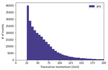
At this point we are ready to analyze the data. To start, we can plot a histogram with the transverse momentum distribution of the jets. For that we first collect all jet momenta in a single list that we can then plot with matplotlib.

import matplotlib.pyplot as plt
import matplotlib.patches as mpatches

jet_pts=[]
for idx,evt in df[b'jet_pt'].iteritems():
    for pt in evt:
        jet_pts.append(pt)

color_jet='darkslateblue'

plt.hist(np.array(jet_pts)/1000, color=color_jet, bins=200)
plt.xlabel('Transverse momentum [GeV]')
plt.ylabel('# of events')
plt.xlim(0,200)
patch_jet = mpatches.Patch(color=color_jet, label='Jets')
plt.legend(handles=[patch_jet])
plt.show()

Since we have all the data conveniently in a DataFrame we can also explore some more. For example we can determine what the ratio between electrons and muons in this run is. Both, electrons and muons are leptons and they are stored in the same feature. To separate them, we just loop over all leptons and sort them by their particle ID. A particle ID of 11 corresponds to an electron, an ID of 13 corresponds to a muon, This is the so called Monte Carlo numbering scheme. Since we are looking at single top production, there should only be one lepton in the event. Therefore we throw away all events with more or less than one lepton. These events are called background events, events that mimic the single top event, but actually have a different underlying physical process. In addition to the sorting, we also save the lepton energy.

electrons=[]
muons=[]
for idx,evt in df[b'lep_type'].iteritems():
    if len(evt)==1:
        lep=evt[0]
        if lep==13:
            muons.append(df[b'lep_E'].values[idx][0])
        elif lep==11:
            electrons.append(df[b'lep_E'].values[idx][0])

Now we have the electrons and muons separated we can determine the ratio.

print("Ratio of electrons over muons: " + str(np.round(len(np.array(electrons))/len(np.array(muons)),decimals=3)))

Ratio of electrons over muons: 1.053

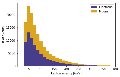
As expected, the ratio is close to one, with a few more electrons. Finally, we can also plot the distribution of the electron and muon energies.

color_el='darkslateblue'
color_mu='goldenrod'

plt.hist([np.array(electrons)/1000, np.array(muons)/1000], bins=80, color=[color_el,color_mu], stacked=True)
plt.xlabel('Lepton energy [GeV]')
plt.ylabel('# of events')
plt.xlim(0,400)
patch_el = mpatches.Patch(color=color_el, label='Electrons')
patch_mu = mpatches.Patch(color=color_mu, label='Muons')
plt.legend(handles=[patch_el,patch_mu])
plt.show()