I got this idea from another blog by Xiang Cao. The idea is to use the power of data analysis to find a job in data science. The question is where you can find a company that sponsors H1-B visas. Xiang Cao uses R to analyses the data. In this article I will use python + pandas to go through a similar analysis with the more recent H1-B disclosure data from the federal fiscal year 2018. For geovisualization of the data I will show two examples using Plotly. This will allow us to see the distribution of employers that sponsor H1-B visas on a US map.</p>
Here I will not go through each step of exploring the data, but rather focus on the important steps that are required to get the results and plots we would like in th end.
import numpy as np
import pandas as pd
import matplotlib.pyplot as plt
First we import the data that comes in form of an Excel spreadsheet. We are not interested in all the available attributes, so let save the relevant ones in a new DataFrame. You can have a look at all the available attributes by typing h1b.keys(). A description of the different attributes can also be found on the homepage. Here, we are specifically interested in the job title, employer name and address and the wage rate. We are also interested in whether the visa was issued as a new employment and whether it is a full time position.
h1b=pd.read_excel("H-1B_Disclosure_Data_FY2018-Q3.xlsx")
h1brel=h1b.loc[:,['JOB_TITLE',
                  'EMPLOYER_NAME','EMPLOYER_ADDRESS','EMPLOYER_CITY','EMPLOYER_STATE','EMPLOYER_POSTAL_CODE',
                  'NEW_EMPLOYMENT',
                  'WAGE_RATE_OF_PAY_FROM','WAGE_UNIT_OF_PAY']]
To clean up the data we need to remove all the NaN values. We can print the number of NaN values per column and the respective data type. Here we choose to replace the string type NaN objects with an empty string and both ‘NEW_EMPLOYMENT’ and ‘WAGE_RATE_OF_PAY_FROM’ with ‘-1’.
print("Number of NaN per column:\n")
print(h1brel.isna().sum())
h1brel['JOB_TITLE'].fillna('', inplace=True)
h1brel['EMPLOYER_NAME'].fillna('', inplace=True)
h1brel['EMPLOYER_ADDRESS'].fillna('', inplace=True)
h1brel['EMPLOYER_CITY'].fillna('', inplace=True)
h1brel['EMPLOYER_STATE'].fillna('', inplace=True)
h1brel['EMPLOYER_POSTAL_CODE'].fillna('', inplace=True)
h1brel['NEW_EMPLOYMENT'].fillna(-1, inplace=True)
h1brel['WAGE_RATE_OF_PAY_FROM'].fillna(-1, inplace=True)
h1brel['WAGE_UNIT_OF_PAY'].fillna('', inplace=True)
Output:
Number of NaN per column:

JOB_TITLE                 2
EMPLOYER_NAME            16
EMPLOYER_ADDRESS          7
EMPLOYER_CITY             7
EMPLOYER_STATE           33
EMPLOYER_POSTAL_CODE     15
NEW_EMPLOYMENT            0
WAGE_RATE_OF_PAY_FROM     0
WAGE_UNIT_OF_PAY          8
dtype: int64
Next, we need to be more precise in defining what kind of jobs we are looking for. To keep it simple we will focus on a few examples, namely data science, data analysis and machine learning jobs. We also want to exclude any academic positions and restrict our analysis on new employment positions.
jobs=h1brel[h1brel['JOB_TITLE'].str.contains("DATA SCIENTIST|DATA SCIENCE|DATA ANALYST|DATA ANALYTICS|MACHINE LEARNING")]
jobs=jobs[~jobs['JOB_TITLE'].str.contains("LECTURER|PROFESSOR|DOCTORAL")]
jobs=jobs[jobs['NEW_EMPLOYMENT']==1]
jobs.reset_index(drop=True, inplace=True)
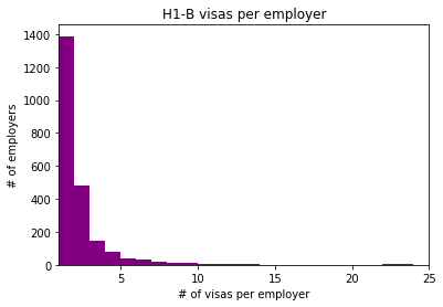
With the data organized we can now turn our focus to the description of that data. For example, we can calculate how many sponsored H1-B visas there are per company. As you can see in the graph below, most companies only support a few H1-B visas. Even more, about 80% of the companies only support one H1-B visa.
import matplotlib.patches as mpatches
h1bperemployer=jobs['EMPLOYER_NAME'].value_counts()
print("There are " + str(len(h1bperemployer)) + " employers in total.")
plt.hist(h1bperemployer.values, bins=range(1, 25),color='purple')
plt.title("H1-B visas per employer")
plt.xlim(1, 25)
plt.xlabel('# of visas per employer')
plt.ylabel('# of employers')
plt.show()
Output:
There are 2261 employers in total.
The H1-B disclosure data also states the wages for the individual positions. Let’s have a look at what this means for data scientists and data analysts, respectively. We only look at the yearly wages here, so we need to filter by WAGE_UNIT_OF_PAY. The average yearly wage of a data scientist is around $100,000, for the data analyst it is a bit less at around $77,000.
datascientists = jobs[jobs['JOB_TITLE'].str.contains("DATA SCIENTIST|DATA SCIENCE")]
datascientistwages=datascientists[datascientists['WAGE_UNIT_OF_PAY'].str.contains("Year")]

analysts = jobs[jobs['JOB_TITLE'].str.contains("DATA ANALYST|DATA ANALYTICS")]
analystwages=analysts[analysts['WAGE_UNIT_OF_PAY'].str.contains("Year")]

purple_patch = mpatches.Patch(color='purple', label='Data Scientists')
teal_patch = mpatches.Patch(color='teal', label='Data Analysts')
plt.legend(handles=[purple_patch,teal_patch])
plt.hist([datascientistwages['WAGE_RATE_OF_PAY_FROM'],analystwages['WAGE_RATE_OF_PAY_FROM']], bins=40,stacked=True, color=['purple','teal'], histtype='stepfilled')
plt.title("Yearly wages of Data Scientists and Data Analysts")
plt.xlim(0, 300000)
plt.xlabel('Wages in USD')
plt.ylabel('# of visas')
plt.show()
print("Mean wages for Data Scientists: $" + str(round(datascientistwages['WAGE_RATE_OF_PAY_FROM'].mean(),ndigits=2)))
print("Mean wages for Data Analysts:   $" + str(round(analystwages['WAGE_RATE_OF_PAY_FROM'].mean(),ndigits=2)))
Output:
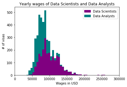
Mean wages for Data Scientists: $100761.28
Mean wages for Data Analysts:   $77357.74
Finally, we would also like to know where the companies that sponsor H1-B visas are located. For that we use the addresses provided and transform those into geolocations, that means geographic coordinates given by latitude and longitude. For each employer we count the number of H1-B visas issued to get a feeling of where the most employers are located.
jobs_unique=jobs.drop_duplicates(subset='EMPLOYER_NAME', keep='first', inplace=False).reset_index(drop=True, inplace=False)
employers_unique=jobs['EMPLOYER_NAME'].value_counts(sort=False)
jobs_unique['COUNT']=""
for idx,js in jobs_unique.iterrows():
    jobs_unique['COUNT'].loc[idx]=employers_unique[js['EMPLOYER_NAME']]
jobs_unique['ADDRESS']=jobs_unique['EMPLOYER_ADDRESS']+", "+jobs_unique['EMPLOYER_CITY']+', '+jobs_unique['EMPLOYER_STATE']+' '+jobs_unique['EMPLOYER_POSTAL_CODE']
Using the OpenStreetMap geocoder we can get the coordinates of each address. This will then allow us to plot the locations on a map.
geolocations=[]
import geocoder
import requests
import logging
import time
logging.basicConfig()
with requests.Session() as session:
    for idx, ad in jobs_unique.iterrows():
        geoc=geocoder.osm(ad['ADDRESS'], session=session)
        if geoc.ok:
            geox=geoc.osm['x']
            geoy=geoc.osm['y']
            geolocations.append([ad['EMPLOYER_NAME'],ad['ADDRESS'],geox,geoy,ad['COUNT']])
        time.sleep(5)

geodf = pd.DataFrame(geolocations,columns=['EMPLOYER_NAME','ADDRESS','lon','lat','COUNT'])
To plot the employers locations on a map we use Plotly, which provides a straightforward way of visualizing geographical data. First we want to use a geographical scatter-plot, where the size and color of a point represents the amount of supported visas at a certain location.
import plotly.plotly as py
import plotly
geodf['text'] = 'Employer: ' + geodf['EMPLOYER_NAME'].astype(str) + '<br>' + 'Address: ' + geodf['ADDRESS'].astype(str) + '<br>' + 'Supports ' + geodf['COUNT'].astype(str) + ' H1-B visas'

limits = [(0,10),(11,50),(51,100),(100,250)]
colors = ["rgb(153, 102, 255)","rgb(0, 153, 255)","rgb(255, 255, 0)","rgb(204, 0, 0)"]
places = []

for i in range(len(limits)):
    lim = limits[i]
    df = geodf[(geodf['COUNT']<=lim[1]) & (geodf['COUNT']>=lim[0])]
    place = dict(
        type = 'scattergeo',
        locationmode = 'USA-states',
        lon = df['lon'],
        lat = df['lat'],
        text = df['text'],
        marker = dict(
            size = 5*df['COUNT'],
            color = colors[i],
            line = dict(width=0.5, color='rgb(40,40,40)'),
            sizemode = 'area'
        ),
        name = '{0} - {1}'.format(lim[0],lim[1]) )
    places.append(place)

layout = dict(
        title = 'H1-B employers in 2018<br>(Click legend to toggle traces)',
        showlegend = True,
        geo = dict(
            scope='usa',
            projection=dict( type='albers usa' ),
            showland = True,
            landcolor = 'rgb(153, 153, 102)',
            subunitwidth=1,
            countrywidth=1,
            subunitcolor="rgb(255, 255, 255)",
            countrycolor="rgb(255, 255, 255)"
        ),
    legend = dict(
           traceorder = 'reversed'
    )
)

fig = dict( data=places, layout=layout )
plotly.offline.plot( fig, validate=False, filename='h1bemployerspercitymap.html' )
Click the image to view and explore the map in full detail!
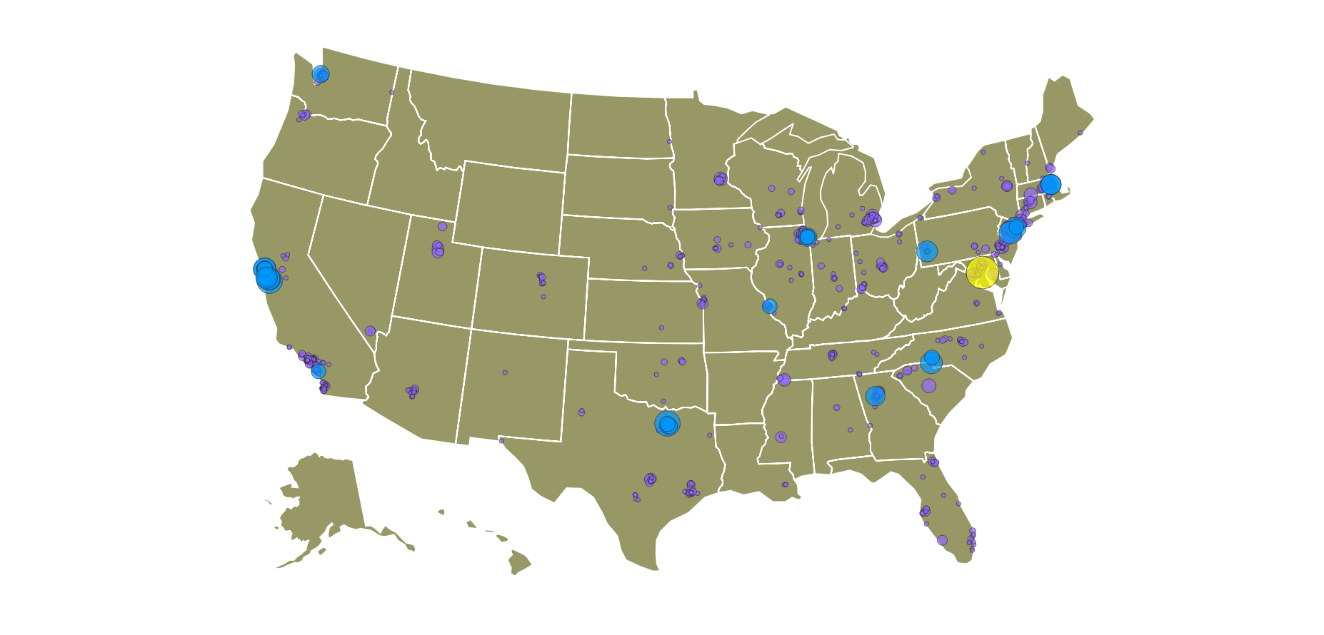
From the map we can see that there are a number of companies that support a large number of visas, like Google, Amazon and the like. Of course this was to be expexted. But now we can also see that a large number of companies that only support one or a few visas is scatter all over the US.
To see in which state the most data science jobs are we can again use Plotly, this time with a choropleth map. We can simply count the number of employers per state given the EMPLOYER_STATE attribute and the tint of the individual states show us how many jobs there are.
jobs_unique_state=jobs.drop_duplicates(subset='EMPLOYER_STATE', keep='first', inplace=False).reset_index(drop=True, inplace=False)
employers_unique_state=jobs['EMPLOYER_STATE'].value_counts(sort=False)
jobs_unique_state['COUNT']=""
for idx,js in jobs_unique_state.iterrows():
    jobs_unique_state['COUNT'].loc[idx]=employers_unique_state[js['EMPLOYER_STATE']]
scl = [[0.0, 'rgb(242,240,247)'],[0.2, 'rgb(218,218,235)'],[0.4, 'rgb(188,189,220)'],\
            [0.6, 'rgb(158,154,200)'],[0.8, 'rgb(117,107,177)'],[1.0, 'rgb(84,39,143)']]

jobs_unique_state['text'] = jobs_unique_state['COUNT'].astype(str) + ' supported H1-B visas'

data = [ dict(
        type='choropleth',
        colorscale = scl,
        autocolorscale = False,
        locations = jobs_unique_state['EMPLOYER_STATE'],
        z = jobs_unique_state['COUNT'].astype(float),
        locationmode = 'USA-states',
        text = jobs_unique_state['text'],
        marker = dict(
            line = dict (
                color = 'rgb(255,255,255)',
                width = 2
            ) ),
        colorbar = dict(
            title = "H1-B visas")
        ) ]

layout = dict(
        title = 'H1-B Employers in 2018 by State<br>(Hover for details)',
        geo = dict(
            scope='usa',
            projection=dict( type='albers usa' ),
            showlakes = True,
            lakecolor = 'rgb(255, 255, 255)'),
             )

fig = dict( data=data, layout=layout )
plotly.offline.plot( fig, filename='h1bemployersperstatemap.html' )
Click the image to view and explore the map in full detail!
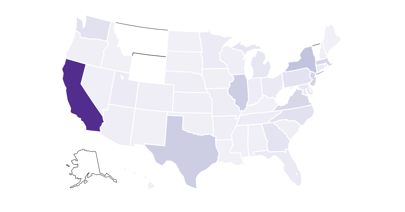
That’s it! Of course it is no surprise that the most data science positions are in California, but there are also a number of places on the east cost that support H1-B visas (and even some states without any H1-B visa supporters). This is certainly some useful information if you’re planing to look for a job in data science.